This tutorial is the final work for the Workshop on Geospatial data processing and analysis using GRASS GIS software organized by Instituto de Altos Estudios Espaciales “MARIO GULICH” (Argentina) taught by Dr. Veronica Andreo
Introduction
Identifying and mapping species across the landscape is crucial to understand the determinants of species distribution and persistence through time. Remote sensing allow researchers to collect continuous RGB, multispectral or hyperspectral data that, allows for species mapping and, even provide information on other species features such stress and water content.
Multiple species classification workflows using a wide range of processing time and precision have been proposed, but with a limited applicability, as most of those methods are computer resources-hungry. The GRASS GIS software provides a robust and efficient platform to perform all the steps of the analyses within the same framework while harnessing the potential of packages developed within GRASS GIS and R. In this tutorial, we exemplify step-by-step the use of GRASS GIS in the classification of species in hyperspectral images using a combination of superpixels, unsupervised segmentation and machine learning.
Hyperspectral Data
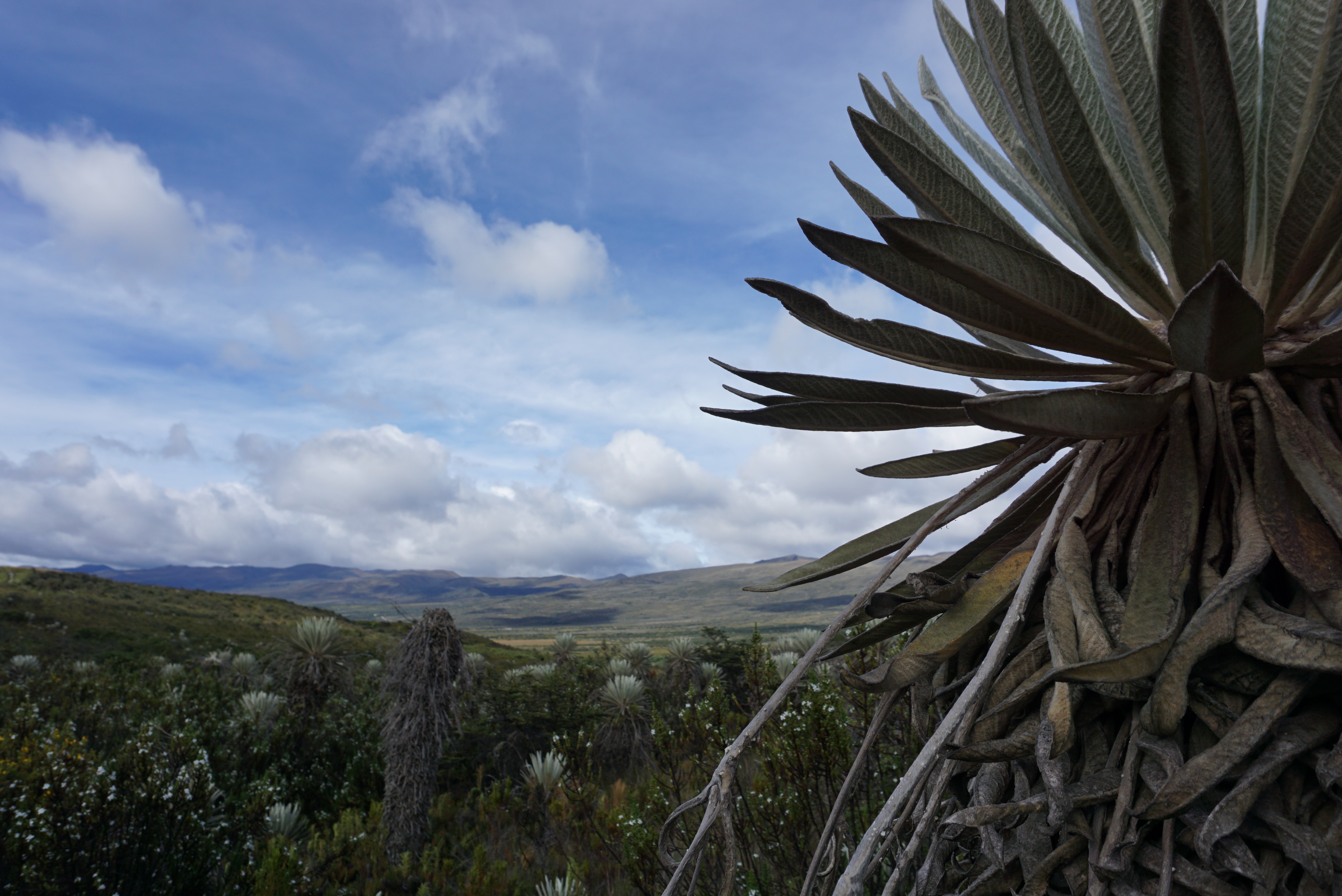
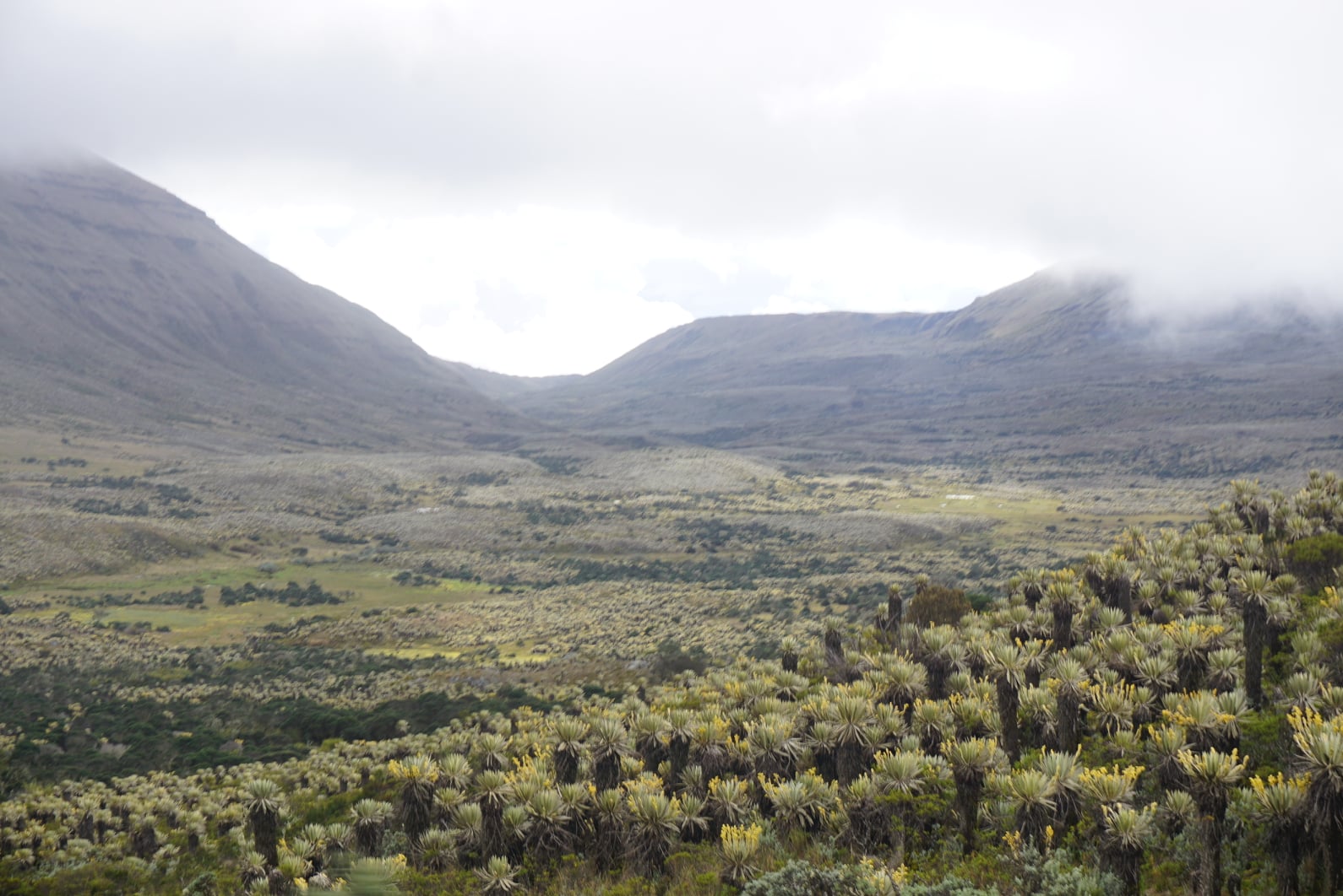
The hyperspectral data used in this tutorial, consists of one image (2Gb size) of 272 bands (2 cm pixel resolution), collected using a UAV (Unnocuppied Aerial Vehicle) taken from a tropical alpine ecosystem known as paramo and located in the highlands of the Colombian Andes. Paramos are characterized by a diverse range or short plants that include grasses, shrubs, mosses and rosettes. This growth forms include an important number of endemic species.
This data is part of a large warming experiment, own and managed by ECOFIV (Plant Ecophysiology lab) at Universidad de los Andes). The use of any of the screenshots and photos provided in this tutorial is stricly prohibited.
Terminology overview
Superpixels
Superpixels algorithm captures image redundancy, and in doing so it groups pixels with similar spectral properties. The advantage of this approach lies in the reduction of the complexity of the image thereby increasing the speed and quality of the analyses. In GRASS GIS, the i.superpixels.slic addon, developed by Rashad Kanavath and Markus Metz, uses the simple linear iterative clustering (SLIC) which is an adaptation of k-means (i.e. clustering technique), that weights the superpixel formation by spectral properties and spatial proximity and has a limited search space (Achanta et al. 2012). Such processes improves the quality and speed of the segmentation process.
Unsupervised Segmentation Parameter Optimization (USPO)
Image segmentation for further object-based image analysis (OBIA) requires the setup of parameters like shape and size of the segments. This process is time consuming and can lead to errors in the segmentation processes. The USPO approach reduces processing time while optimizing parameter selection using the spectral properties of the image (Johnson et al, 2015). In GRASS GIS this feature is found in the i.segment.uspo add-on, developed by Moritz Lennert.
Machine learning
A range of machine learning algorithms (e.g. random forest, support vector machines, etc) are currently widely used for species/land cover image classification and have been implemented. The caret R package provides a set of tools and options that allow tuning and testing multiple approaches for a robust classification. The caret package can be use within GRASS GIS thanks to the add-on _ v.class.mlR_, developed by Moritz Lennert and based on a R script written by Ruben Van De Kerchove. It is a simple yet efficient and robust module for image classification.
Software required
This tutorial is performed in Linux Fedora 33.
We will use the following software and packages:
- GRASS GIS 7.85
- GRASS GIS addons
g.extension i.superpixels.slic
g.extension r.neighborhoodmatrix
g.extension i.segment.uspo
g.extension i.segment.stats
g.extension r.object.geometry
g.extension v.class.mlR
- R Software
- R packages:
install.packages("caret","ggplot2","foreach", \
"iterators","parallel")
Workflow overview
In this tutorial we will:
- Import raster and vector files
- Set up the computational region and mask for further processes
- Calculate spectral indices based on the hyperspectral Data
- Run the superpixels module
- Run the unsupervised segmentation optimization parameter optimization (USPO)
- Image classification using machine learning
- Accuracy Assessment
Import raster and vector files
Import hyperspectral data (tif format)
r.in.gdal input=New_18342/raw_18342_rd_rf_W_modified.tif \
output=raw_1834_modified
You can see the spectral signature of the image by selecting an area of the map and copying the coordinates of that location by right-clicking on to the map and selecting copy coordinates to clipboard then paste the coordinates in the command line:
i.spectral -g group=raw_18342_rd_rf_W_modified coordinates=-73.99236321556138,4.550556320042415

Import vector data (random points used for training and testing the classification, and a image boundary to use as a mask)
v.in.ogr --overwrite input=New_18342/POL_19_FAR_points.shp \
layer=POL_19_FAR_points output=POL_19_FAR_points
v.in.ogr --overwrite input=New_18342/blocks3.shp layer=blocks3 \
output=blocks3
v.in.ogr --overwrite input=New_18342/rand_point18342.shp \
layer=rand_point18342 output=rand_point18342
Set up computational region and mask
Use the raster to align region to one of the raster bands
g.region -p raster=raw_18342_rd_rf_W_modified.1 save=paramo_full
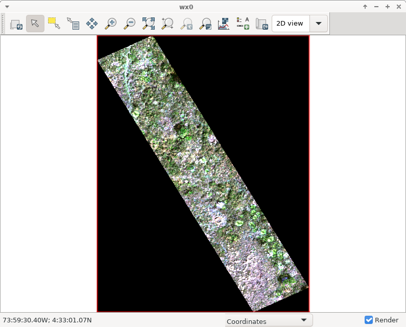
Display RGB image of the raster
d.mon wx0
d.rgb red=raw_18342_rd_rf_W_modified.38 green=raw_18342_rd_rf_W_modified.65 \
blue=raw_18342_rd_rf_W_modified.127

Use i.colors.enhance to enhance image contrast
i.colors.enhance red=raw_18342_rd_rf_W_modified.38 \
green=raw_18342_rd_rf_W_modified.65  blue=raw_18342_rd_rf_W_modified.127 -r
r.mask vector=blocks3
check for NULL values in one band
r.univar -e raw_18342_rd_rf_W_modified.38 percentile=98

Create a group containing image bands
i.group group=RF_18342 input= `g.list raster, \
pattern="raw_18342_rd_rf_W_modified*`
Calculate spectral indices based on the hyperspectral Data
Estimate vegetation index using the i.vi module
i.vi output=raw_18342_vi_NDVI viname=ndvi \
red=raw_18342_rd_rf_W_modified.124 nir=raw_18342_rd_rf_W_modified.194

r.univar -e raw_18342_vi_NDVI percentile=98

The same results are obtain writing the NDVI equation using the module r.mapcalc
r.mapcalc "ndvi_18342 = float(raw_18342_rd_rf_W_modified.194 - \
raw_18342_rd_rf_W_modified.124)/(raw_18342_rd_rf_W_modified.194 +  \
raw_18342_rd_rf_W_modified.124)" --o

r.univar -e ndvi_18342 percentile=98

Calculate Red edge chlorophyll index (CI)
r.mapcalc "RedEdge_18342 = float(raw_18342_rd_rf_W_modified.160 \
  raw_18342_rd_rf_W_modified.142)"  --o

Calculate Optimized Soil Adjusted Vegetation Index (OSAVI)
r.mapcalc "OSAVI_18342 = float(((1+0.16)* \
(raw_18342_rd_rf_W_modified.182-raw_18342_rd_rf_W_modified.124))/(raw_18342_rd_rf_W_modified.182+raw_18342_rd_rf_W_modified.124+0.16))" --o

Calculate Structure Intensive pigment Index (SIPI)
r.mapcalc "sipi_18342 = float(raw_18342_rd_rf_W_modified.182 - \
raw_18342_rd_rf_W_modified.24) / (raw_18342_rd_rf_W_modified.182 + \
raw_18342_rd_rf_W_modified.24)" --o

Run the superpixels module
You must have already installed the i.superpixels.slic add-on.
Run superpixels to use as seeds for the USPO procedure
i.superpixels.slic input=RF_18342group output=superpixelsRF1 \
 step=2 compactness=0.7 memory=2000`

r.info superpixelsRF1
Run the unsupervised segmentation optimization parameter optimization (USPO)
Remember to have the r.neighborhoodmatrix and i.segment.uspo addons installed.
Run segmentation with uspo using the superpixels output as the seeds.
i.segment.uspo group=RF_18342group
               output=uspo_parameters.csv
               region=paramo_full
               seeds=superpixelsRF1
               segment_map=segsRF1
               threshold_start=0.005
               threshold_stop=0.05
               threshold_step=0.05
               minsizes=1,3,5,6,7
               number_best=5
               memory=2000 processes=4 --o

r.to.vect -tv input=segsRF_paramo_full_rank1 output=segsRF1 type=area

Extract stats of the spectral indices for the segments
i.segment.stats map=segsRF_paramo_full_rank1
                rasters=ndvi_18342,RedEdge_18342,OSAVI_18342,sipi_18342
                raster_statistics=mean,stddev
                area_measures=area,perimeter,compact_circle,compact_square
                vectormap=segsRF_stats
                processes=4 --o

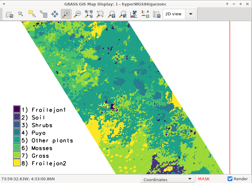
Image classification using machine learning
Use ground truth points and label them
v.info rand_point18342
Number of points per class
db.select \
  sql="SELECT classtype,COUNT(cat) as count_class
       FROM rand_point18342
       GROUP BY classtype"
Select segments that are below the training points
v.select ainput=segsRF_stats
         binput=rand_point18342
         output=train_segments
         operator=overlap --o
Get the information regarding the segments under the points and use them as training set
v.info train_segments
Add a column to train segments to assign a label from the training points
v.db.addcolumn train_segments column="class int"

v.distance from=train_segments
           to=rand_point18342
           upload=to_attr
           column=class
           to_column=classtype
Group training segments per class
db.select \
  sql="SELECT class,COUNT(cat) as count_class
       FROM train_segments
       GROUP BY class"
You must have the v.class.mlR add-on already installed. Previous to this step, remember to open R (or Rstudio) and installed the R packages listed at the beginning of this tutorial, you can copy paste the script provided.
Run the classification using the Random forest machine learning algorithm as the classifier.
v.class.mlR -nf   segments_map=segsRF1_stats
                  training_map=train_segments
                  train_class_column=class
                  output_class_column=class_rf1
                  classified_map=classification1
                  raster_segments_map=segsRF1_paramo_full_rank1
                  classifier=rf
                  folds=5
                  partitions=10
                  tunelength=10
                  weighting_modes=smv
                  weighting_metric=accuracy
                  output_model_file=model
                  variable_importance_file=var_imp.txt
                  accuracy_file=accuracy.csv
                  classification_results=all_resultsRF1.csv
                  model_details=classifier_runs.txt
                  r_script_file=Rscript_mlR.R
                  processes=4 --o
Variable importance is stored in a txt file:
Classifier: rf******************************            Overall
OSAVI_18342_mean     100.000000
sipi_18342_mean       91.907236
RedEdge_18342_mean    81.265406
ndvi_18342_mean       51.628978
OSAVI_18342_stddev    32.834966
ndvi_18342_stddev     29.512831
sipi_18342_stddev     27.098430
RedEdge_18342_stddev  25.222485
area                  15.178810
perimeter              4.550482
compact_square         2.119414
compact_circle         0.000000
Accuracy Assessment
Validation of the classification using the testing set of points
v.info POL_19_FAR_points

db.select \
  sql="SELECT clastype,COUNT(cat) as count_class
       FROM POL_19_FAR_points
       GROUP BY clastype"
Select segments that are below testing points
v.select ainput=segsRF_stats binput=POL_19_FAR_points output=test_segments operator=overlap --o

v.info test_segments
Add column to the testing segments
v.db.addcolumn test_segments column="class int"
Assign label from testing points to segments
v.distance from=test_segmentsRF1
          to=POL_19_FAR_points
          upload=to_attr
          column=class
          to_column=classtype
Convert testing segments to raster to be compared with the results of the classification
v.to.rast input=test_segments use=attr attribute_column=class output=testing
Create confusion matrix and estimate precision measures
r.kappa classification=classification_rf reference=testing
ACCURACY ASSESSMENT
LOCATION: hyperWGS84				Wed Apr 14 12:08:35 2021
MASK: MASK in garzonc
MAPS: MAP1 = Categories (testingRF1 in garzonc)
MAP2 = Reclass of segsRF1_paramo_full_rank1 in garzonc (classification1_rf in garzonc)

Error Matrix (MAP1: reference, MAP2: classification)
Panel #1 of 2
  MAP1
cat#	1	2	4	5	6
M     1	1074	0	0	0	0
A     2	0	0	0	0	0
P     4	248	0	20868	0	0
2     5	3369	0	843	0	0
 6	468	0	0	0	20502
 7	8065	0	2330	0	8378
 8	0	0	0	0	9306
Col Sum		13224	0	24041	0	38186

Panel #2 of 2
  MAP1
cat#	7	8	Row Sum
M     1	0	0	1074
A     2	0	13358	13358
P     4	0	0	21116
2     5	27833	74	32119
 6	188	0	21158
 7	21582	18706	59061
 8	0	2651	11957
Col Sum		49603	34789	159843


Cats	% Comission	% Omission	Estimated Kappa
1	0.000000	91.878403	1.000000
2	NA		NA		NA
4	1.174465	13.198286	0.986176
5	NA		NA		NA
6	3.100482	46.310166	0.959263
7	63.458120	56.490535	0.079886
8	77.828887	92.379775	0.005198

Kappa		Kappa Variance
0.286594	0.000002

Obs Correct	Total Obs	% Observed Correct
66677		159843		41.714057
This tutorial was developed using a simplify set of options with basic levels of testing and tuning. Higher accuracy is expected as tests with varying parameters and algorithms are performed in order to produced better-tuned models. It is still an extremely good outcome to reach such accuracy for species classification with this unsupervised approach in such a diverse ecosystem with short species and in no more than 1 hour of total processing time.
I personally look forward to continue to learn about GRASS GIS and gain expertise using its add-ons! I feel compelled show my appreciation to the GRASS GIS community for the development of such useful OpenSource software and tools, and their never ending support to researchers worldwide.